Area/Geometry Problem

This problem is from The Geometry Forum Problem of the Week June 1996

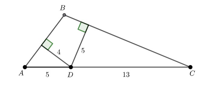
In triangle ABC, AC=18 and D is the point on AC for which AD=5. Perpendiculars drawn from D to AB and CB have lengths of 4 and 5 respectively. What is the area of triangle ABC?

I put together a diagram (in Geogebra)
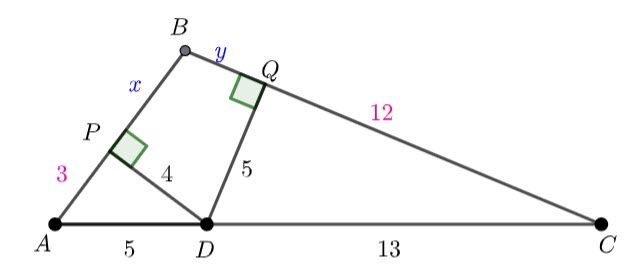
Add points P and Q

Triangle APD and triangle DQC are right angled. Using pythagoras, AP=3 and QC=12

BQDP is a cyclic quadrilateral and BD is the diameter. I am not sure if this is useful, but it is good to notice.
    \begin{equation*}sin(A+B+C)=sin(180)=0\end{equation}

    \begin{equation*}sin((A+C)+B)=sin(A+C)cosB+sinBcos(A+C)=0\end{equation}

    \begin{equation*}cosB(sinAcosC+sinCcosA)+sinB(cosAcosC-sinAsinC)=0\end{equation}

    \begin{equation*}cosB(\frac{4}{5}\times\frac{12}{13}+\frac{5}{13}\times\frac{3}{5})+sinB(\frac{3}{5}\times\frac{12}{13}-\frac{4}{5}\times\frac{5}{13})=0\end{equation}

    \begin{equation*}cosB(\frac{48}{65}+\frac{15}{65})+sinB(\frac{36}{65}-\frac{20}{65})=0\end{equation}

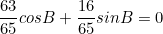
    \begin{equation*}\frac{63}{65}cosB+\frac{16}{65}sinB=0\end{equation}

    \begin{equation*}63cosB+16sinB=0\end{equation}

    \begin{equation*}63+16tanB=0\end{equation}

    \begin{equation*}tanB=\frac{-63}{16}\end{equation}

If tanB=\frac{-63}{16} then sinB=\frac{63}{65}

Now,

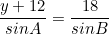
    \begin{equation*}\frac{y+12}{sinA}=\frac{18}{sinB}\end{equation}

    \begin{equation*}y+12=\frac{4}{5}(18)\frac{65}{63}\end{equation}

    \begin{equation*}y+12=\frac{104}{7}\end{equation}

Hence the Area is

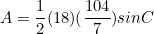
    \begin{equation*}A=\frac{1}{2}(18)(\frac{104}{7})sinC\end{equation}

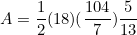
    \begin{equation*}A=\frac{1}{2}(18)(\frac{104}{7})\frac{5}{13}\end{equation}

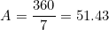
    \begin{equation*}A=\frac{360}{7}=51.43\end{equation}

Leave a Comment

Filed under Area, Finding an area, Geometry, Identities, Non-Right Trigonometry, Pythagoras, Trigonometry

Binomial Expansion – deriving the formula for Variance

We have seen how the formula for mean (expected value) was derived, and now we are going to look at variance.

In general variance of a probability distribution is

(1)   \begin{equation*} Var(X)=E(X^2)-(E(X))^2\end{equation*}

We are going to start by calculating E(X^2)

    \begin{equation*}E(X^2)=\sum_{x=0}^nx^2p(x)\end{equation}

    \begin{equation*}E(X^2)=\sum_{x=0}^nx^2\begin{pmatrix}n\\x\end{pmatrix}p^x(1-p)^{n-x}\end{equation}

    \begin{equation*}E(X^2)=\sum_{x=0}^n x^2\frac{n!}{(n-x)!x!}p^x(1-p)^{n-x}\end{equation}

The x^2 cancels with the x! to leave x on the numerator and (x-1)! on the denominator.

Also, when x=0, x^2=0 and we can start the sum at x=1

    \begin{equation*}E(X^2)=\sum_{x=1}^n x\frac{n!}{(n-x)!(x-1)}!p^x(1-p)^{n-x}\end{equation}

Let y=x-1 and m=n-1, when x=n, y=n-1 and hence y=m and when x=1, y=0

Our equation is now

    \begin{equation*}E(X^2)=\sum_{y=0}^m (y+1)\frac{(m+1)!}{(m+1-(y+1))!y!}p^{y+1}(1-p)^{m+1-(y+1)}\end{equation}

Simplify

    \begin{equation*}E(X^2)=\sum_{y=0}^m(y+1)\frac{(m+1)!}{(m-y)!y!}p^{y+1}(1-p)^{m-y}\end{equation}

    \begin{equation*}E(X^2)=\sum_{y=0}^m(y+1)(m+1)\frac{m!}{(m-y)!y!}p\times p^y(1-p)^{m-y}\end{equation}

    \begin{equation*}E(X^2)=\sum_{y=0}^m p(y+1)(m+1)\frac{m!}{(m-y)!y!} p^y(1-p)^{m-y}\end{equation}

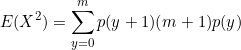
    \begin{equation*}E(X^2)=\sum_{y=0}^m p(y+1)(m+1)p(y)\end{equation}

    \begin{equation*}E(X^2)=p(m+1)(\sum_{y=0}^myp(y)+\sum_{y=0}^mp(y))\end{equation}

\sum_{y=0}^mp(y)=1 and \sum_{y=0}^myp(y)=E(Y)

    \begin{equation*}E(X^2)=p(m+1)(E(Y)+1)\end{equation}

E(Y)=mp

    \begin{equation*}E(X^2)=p(m+1)(mp+1)\end{equation}

m+1=n

    \begin{equation*}E(X^2)=pn((n-1)p+1)\end{equation}

    \begin{equation*}E(X^2)=n^2p^2-np^2+np\end{equation}

Now from equation 1

    \begin{equation*}Var(X)=E(X^2))-(E(X))^2\end{equation}

    \begin{equation*}=Var(X)=n^2p^2-np^2+np-n^2p^2\end{equation}

    \begin{equation*}Var(X)=-np^2+np\end{equation}

(2)   \begin{equation*}Var(X)=np(1-p)\end{equation*}

and the standard deviation is

(3)   \begin{equation*}\sigma_X=\sqrt{np(1-p)}\end{equation*}

1 Comment

Filed under Algebra, Binomial, Probability Distributions, Standard Deviation

Binomial Distribution – deriving the equation for mean (expected value)

The mean, \mu of a binomial distribution is

(1)   \begin{equation*}\mu=np\end{equation*}

where n is the number of trials and p is the probability of success.

For any discrete probability distribution , the expected value or mean is

(2)   \begin{equation*}E(X)=\sum_{x=0}^nxp(x)\end{equation*}

For example, if a coin is tossed 3 times and the number of heads is recorded, the distribution is

X0123
P(X=x)\frac{1}{8}\frac{3}{8}\frac{3}{8}\frac{1}{8}

    \begin{equation*}E(X)=0\times\frac{1}{8}+1\times\frac{3}{8}+2\times\frac{3}{8}+3\times{1}{8}\end{equation}

    \begin{equation*}E(X)=\frac{12}{8}=\frac{3}{2}\end{equation}

I want to show how the \mu=np formula is derived from the general formula (equation (2)).

    \begin{equation*}E(X)=\sum^n_{x=0}xp(x)\end{equation}

For a binomial distribution, p(x)=\begin{pmatrix}n\\x\end{pmatrix}p^x(1-p)^{n-x}

    \begin{equation*}E(X)=\sum_{x=0}^nx\begin{pmatrix}n\\x\end{pmatrix}p^x(1-p)^{n-x}\end{equation}

    \begin{equation*}E(X)=\sum^n_{x=0}x\frac{n!}{(n-x)!x!}p^x(1-p)^{n-x}\end{equation}

The x can cancel with the x! to leave (x-1)! on the denominator.

    \begin{equation*}E(X)=\sum^n_{x=0}\frac{n!}{(n-x)!(x-1)!}p^x(1-p)^{n-x}\end{equation}

Also, when x=0 \Rightarrow xp(x)=0, hence the sum can start at x=1.

    \begin{equation*}E(X)=\sum^n_{x=1}\frac{n!}{(n-x)!(x-1)!}p^x(1-p)^{n-x}\end{equation}

Let y=x-1 and m=n-1

When x=n \Rightarrow y=n+1=m

    \begin{equation*}E(X)=\sum^{m}_{y=0}\frac{(m+1)!}{((m+1)-(y+1))!(y)!}p^{y+1}(1-p)^{(m+1)-(y+1)}\end{equation}

Simplify

    \begin{equation*}E(X)=\sum^{m}_{y=0}\frac{(m+1)!}{((m-y))!(y)!}p^{y+1}(1-p)^{(m-y)}\end{equation}

    \begin{equation*}E(X)=\sum^{m}_{y=0}\frac{(m+1)m!}{((m-y))!(y)!}p^yp^1(1-p)^{(m-y)}\end{equation}

We can move (m+1) and p out of the sum.

    \begin{equation*}E(X)=(m+1)p\sum^{m}_{y=0}\frac{m!}{((m-y))!(y)!}p^y(1-p)^{(m-y)}\end{equation}

    \begin{equation*}\sum^{m}_{y=0}\frac{m!}{((m-y))!(y)!}p^y(1-p)^{(m-y)}=\sum^{m}_{y=0}\begin{pmatrix}m\\y\end{pmatrix}p^y(1-p)^{(m-y)}\end{equation}

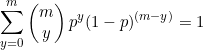
    \begin{equation*}\sum^{m}_{y=0}\begin{pmatrix}m\\y\end{pmatrix}p^y(1-p)^{(m-y)}=1\end{equation}

As it is the sum of the probabilities of a binomial distribution with m trials.

Hence E(X)=(m+1)p=np

Next, deriving the variance formula for a binomial distribution.

1 Comment

Filed under Binomial, Mean, Probability Distributions

Vector and Scalar Projection

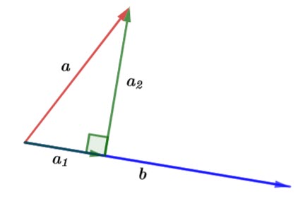
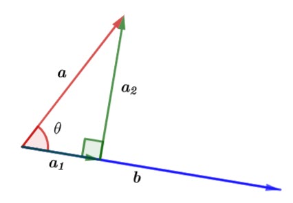
The vector projection (vector resolution or vector component) of \mathbf{a} onto a non-zero vector \mathbf{b} is splitting \mathbf{a} into two vectors, one is parallel to \mathbf{b} (the vector projection) and one perpendicular to \mathbf{b}

In the above diagram \mathbf{a_1} is the vector projection of \mathbf{a} onto \mathbf{b} and \mathbf{a_2} is perpendicular to \mathbf{b}.

How do we find \mathbf{a_1} and \mathbf{a_2}?

Using right trigonometry,

cos(\theta)=\frac{|\mathbf{a_1}|}{|\mathbf{a}|}

Remember the scalar product (dot product) of vectors is

(1)   \begin{equation*}\mathbf{a}\cdot\mathbf{b}=|\mathbf{a}||\mathbf{b}|cos(\theta)\end{equation*}

Hence cos(\theta)=\frac{\mathbf{a}\cdot\mathbf{b}}{|\mathbf{a}||\mathbf{b}|}

\frac{\mathbf{a}\cdot\mathbf{b}}{|\mathbf{a}||\mathbf{b}|}=\frac{|\mathbf{a_1}|}{|\mathbf{a}|}

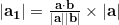
and, |\mathbf{a_1}|=\frac{\mathbf{a}\cdot\mathbf{b}}{|\mathbf{a}||\mathbf{b}|}\times|\mathbf{a}|

|\mathbf{a_1}|=\frac{\mathbf{a}\cdot\mathbf{b}}{|\mathbf{b}|}

This is the scalar projection of \mathbf{a} onto \mathbf{b}

To find the vector projection we need to multiply by \mathbf{\hat{b}}, that is find a vector with the same magnitude as \mathbf{a_1} in the direction of \mathbf{b}.

The vector projection is

\mathbf{a_1}=\frac{\mathbf{a}\cdot\mathbf{b}}{|\mathbf{b}|}\times \mathbf{\hat{b}}

\mathbf{a_1}=\frac{\mathbf{a}\cdot\mathbf{b}}{|\mathbf{b}|}\times \frac{\mathbf{b}}{|\mathbf{b}|}

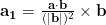
\mathbf{a_1}=\frac{\mathbf{a}\cdot\mathbf{b}}{(|\mathbf{b}|)^2}\times \mathbf{b}

Now for \mathbf{a_2}, we know \mathbf{a}=\mathbf{a_1}+\mathbf{a_2}

Hence, \mathbf{a_2}=\mathbf{a}-\mathbf{a_1}

Example

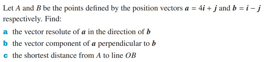
From Cambridge Year 11 Specialist Mathematics (Chapter 3)

(a) \frac{\mathbf{a}\cdot\mathbf{b}}{|\mathbf{b}|^2}\mathbf{b}

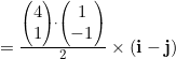
=\frac{\begin{pmatrix}4\\1\end{pmatrix}\cdot\begin{pmatrix}1\\-1\end{pmatrix}}{2}\times(\mathbf{i}-\mathbf{j})

=\frac{3}{2}{(\mathbf{i}-\mathbf{j})

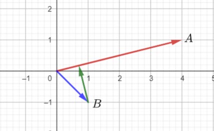
(b)4\mathbf{i}+\mathbf{j}-\frac{3}{2}{(\mathbf{i}-\mathbf{j})=\frac{5}{2}\mathbf{i}+\frac{5}{2}\mathbf{j}

(c)

The shortest distance (green vector) is the vector component of \mathbf{a} perpendicular to \mathbf{b}, i.e. \frac{5}{2}\mathbf{i}+\frac{5}{2}\mathbf{j}

|\frac{5}{2}\mathbf{i}+\frac{5}{2}\mathbf{j}|=\sqrt{\frac{25}{4}+\frac{25}{4}}=\sqrt{\frac{50}{4}}=\frac{5\sqrt{2}}{2}

Leave a Comment

Filed under Right Trigonometry, Trigonometry, Vector Projection, Vectors, Year 11 Specialist Mathematics

Using a Vector Method to Find an Angle Bisector

Points A and B are defined by the position vectors \mathbf{a}=3\mathbf{i}+4\mathbf{j} and \mathbf{b}=12\mathbf{i}+5\mathbf{j}.

Find a vector that bisects \angle{AOB}.

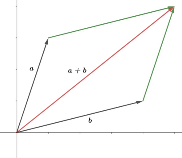
If we think about how we add vectors using the parallelogram rule

Finding the resultant vector using the parallelogram rule

we can take advantage of the geometric properties of parallelograms (or of a rhombus).

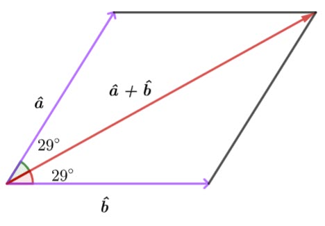
If \mathbf{a} and \mathbf{b} are unit vectors, then the parallelogram is a rhombus, and the diagonal (i.e the resultant) bisects the angle.

We need to find the sum of the unit vectors.

|\mathbf{a}|=\sqrt{3^2+4^2}=5

\therefore \hat{\mathbf{a}}=\frac{3}{5}\mathbf{i}+\frac{4}{5}\mathbf{j}

|\mathbf{b}|=\sqrt{12^2+5^2}=13

\therefore \hat{\mathbf{b}}=\frac{12}{13}\mathbf{i}+\frac{5}{13}\mathbf{j}

The vector that bisects \angle{AOB} is

\frac{3}{5}\mathbf{i}+\frac{4}{5}\mathbf{j}+\frac{12}{13}\mathbf{i}+\frac{5}{13}\mathbf{j}=\frac{99}{65}\mathbf{i}+\frac{64}{65}\mathbf{j}

Leave a Comment

Filed under Geometry, Vectors, Year 11 Specialist Mathematics

Area of Regular Polygons

Finding the area of a regular polygon when you know the side length

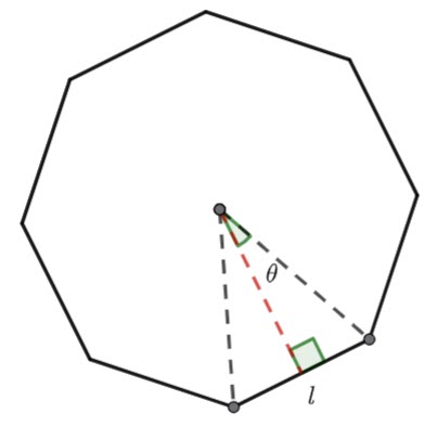
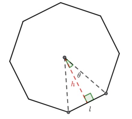
Find the area of an n-sided regular polygon if you know the side length, l.

An octagon for a visual reference

Find the h of the triangle in terms of l and theta.

tan(\theta)=\frac{\frac{l}{2}}{h}

h=\frac{l}{2tan(\theta)}

Remember the area of a triangle is A=\frac{1}{2}bh

Hence, A=\frac{1}{2} l \times \frac{l}{2tan(\theta)}=\frac{l^2}{4tan(\theta)}

And \theta=\frac{360}{2n}=\frac{180}{n}

Therefore A=\frac{l^2}{4tan(\frac{180}{n})}

There are n triangles in an n-sided polygon

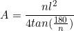
(1)   \begin{equation*}A=\frac{nl^2}{4tan(\frac{180}{n})}\end{equation*}

Find the area of a hexagon with side length 10cm.
A=\frac{6\times10^2}{4tan(\frac{180}{6})}
A=\frac{600}{4(\frac{1}{\sqrt{3}})}
A=150\sqrt{3} cm^2

Finding the area of a polygon if you know the inradius or the apothem

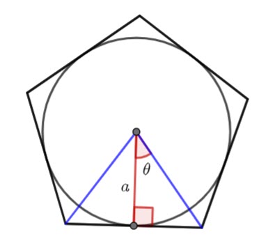
The apothem and the inradius are the same. It is the radius of the incircle.

Find the area of the triangle in terms of a and theta.

tan(\theta)=\frac{\frac{l}{2}}{a}

l=2atan(\theta)

A=\frac{1}{2}bh

A=\frac{1}{2}2atan(\theta)a=a^2tan(\theta)

And \theta=\frac{180}{n}

Hence for an n-sided polygon

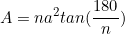
(2)   \begin{equation*}A=na^2tan(\frac{180}{n})\end{equation*}

Find the area of a regular pentagon with apothem 4.5cm
A=5\times 4.5^2tan(\frac{180}{5})
A=73.56cm^2

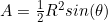
Finding the area of a regular polygon given the circumradius

The circumradius is the radius of the circumscribed circle (R in the diagram above)

Remember the area of triangle formula

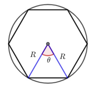
A=\frac{1}{2}absin(\theta)

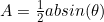
A=\frac{1}{2}R^2sin(\theta)

\theta=\frac{360}{n}

Hence, A=\frac{1}{2}R^2sin(\frac{360}{n})

Hence, for an n-sided polygon

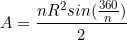
(3)   \begin{equation*}A=\frac{nR^2sin(\frac{360}{n})}{2}\end{equation*}

Find the area of a regular octagon inscribed in a circle of radius 10cm.
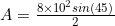
A=\frac{8\times 10^2sin(45)}{2}
A=200\sqrt{2}cm^2

Leave a Comment

Filed under Area, Area of Triangles (Sine), Finding an area, Non-Right Trigonometry, Regular Polygons, Right Trigonometry, Year 11 Mathematical Methods

Deriving the Quadratic Equation formula

My year 10 students have been learning how to complete the square with the idea of then deriving the quadratic equation formula.

The general equation for a quadratic is y=ax^2+bx+c

Completing the square,

    \begin{equation*}ax^2+bx+c\end{equation}

Factorise out the leading coefficient (i.e. a)

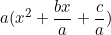
    \begin{equation*}a(x^2+\frac{bx}{a}+\frac{c}{a})\end{equation}

Half the second term (i.e \frac{b}{a}) and subtract the square of the second term.

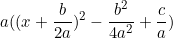
    \begin{equation*}a((x+\frac{b}{2a})^2-(\frac{b}{2a})^2+\frac{c}{a})\end{equation}

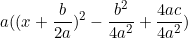
    \begin{equation*}a((x+\frac{b}{2a})^2-\frac{b^2}{4a^2}+\frac{c}{a})\end{equation}

Simplify

    \begin{equation*}a((x+\frac{b}{2a})^2-\frac{b^2}{4a^2}+\frac{4ac}{4a^2})\end{equation}

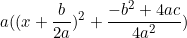
    \begin{equation*}a((x+\frac{b}{2a})^2+\frac{-b^2+4ac}{4a^2})\end{equation}

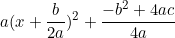
    \begin{equation*}a(x+\frac{b}{2a})^2+\frac{-b^2+4ac}{4a}\end{equation}

Now let’s solve

    \begin{equation*}a(x+\frac{b}{2a})^2+\frac{-b^2+4ac}{4a}=0\end{equation}

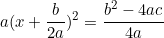
    \begin{equation*}a(x+\frac{b}{2a})^2=\frac{b^2-4ac}{4a}\end{equation}

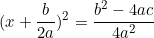
    \begin{equation*}(x+\frac{b}{2a})^2=\frac{b^2-4ac}{4a^2}\end{equation}

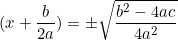
    \begin{equation*}(x+\frac{b}{2a})=\pm \sqrt{\frac{b^2-4ac}{4a^2}}\end{equation}

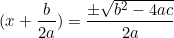
    \begin{equation*}(x+\frac{b}{2a})=\frac{\pm \sqrt{b^2-4ac}}{2a}\end{equation}

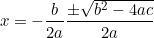
    \begin{equation*}x=-\frac{b}{2a}\frac{\pm \sqrt{b^2-4ac}}{2a}\end{equation}

Which is the quadratic equation formula.

1 Comment

Filed under Algebra, Quadratic, Quadratics, Solving, Solving, Solving Equations

Logistic Growth Worked Example

A brumby is a free-roaming wild horse found in large number in parts of Australia. The culling of brumbies was banned in the year 2000. At this time the estimated population of brumbies in
Kosciuszko National Park was 1600. Scientists have modelled the population, P(t), of brumbies in
Kosciuszko National Park t years since the ban, by

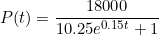
    \begin{equation*}P(t)=\frac{18000}{10.25e^{0.15t}+1}\end{equation}

(a) Use the model to determine how long it will take the brumbies to increase to a number that is triple the number when the ban came into effect.

(b) From this model, determine the estimated long run number of brumbies in Kosciuszko National Park.

It can be shown that the growth rate of the population of brumbies can be expressed as

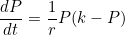
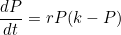
    \begin{equation*}\frac{dP}{dt}=\frac{1}{r}P(k-P)\end{equation}

(c) Determine the values of the constants r and k.

(d) Determine the greatest growth rate for the population of brumbies.

ATAR 2024 Specialist Mathematics Question 13

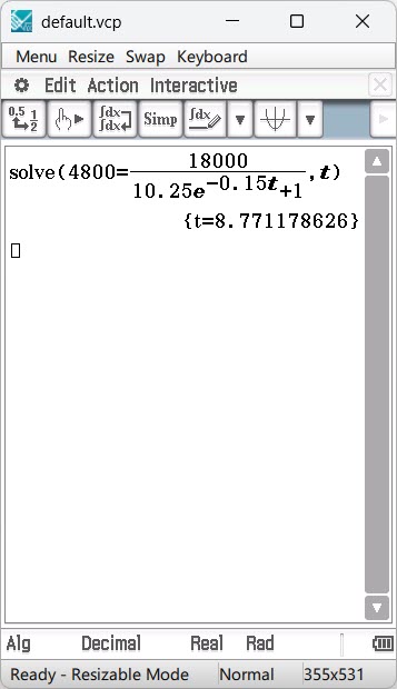
(a) 1600\times 3=4800
4800=\frac{18000}{10.25e^{0.15t}+1}
t=8.8 years.

(b) \lim_{\limits_{t \to \infty}\frac{18000}{10.25e^{0.15t}+1}=18000

(c)k is the carrying capacity (long run number of Brumbies), therefore k=18000.
Remember,

    \begin{equation*}\frac{dP}{dt}=rP(k-P)\Longleftrightarrow P=\frac{KP_0}{(k-P_0)e^{-rkt}+P_0}\end{equation}

We have \frac{1}{r} instead of r.

Therefore,

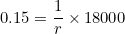
    \begin{equation*}0.15=\frac{1}{r}\times 18000\end{equation}

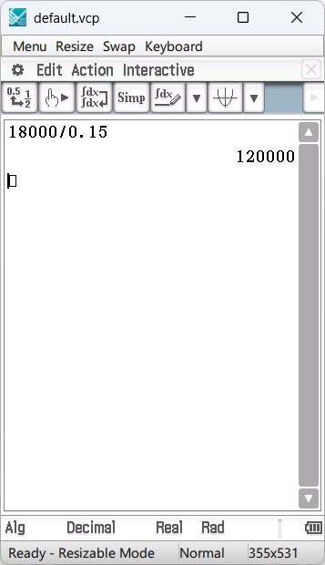
r=120000

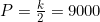
(d) The greatest growth rate occurs when P=\frac{k}{2}=9000

    \begin{equation*}\frac{dP}{dt}=\frac{1}{r}P(k-P)\end{equation}

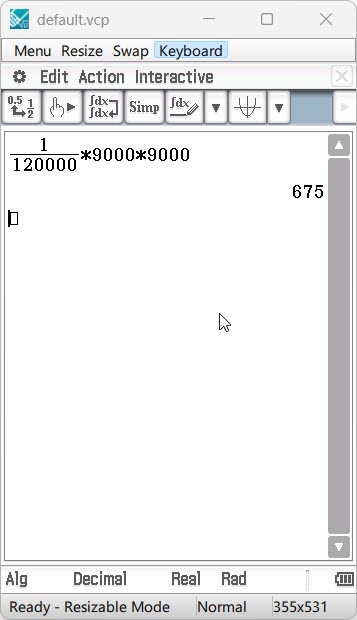
    \begin{equation*}\frac{dP}{dt}=\frac{1}{120000}(9000)(9000)\end{equation}

The greatest growth rate is 675 Brumbies per year.

1 Comment

Filed under Differential Equations, Logistic Growth, Year 12 Specialist Mathematics

Deriving the Logistic Growth Equation

The logistic differential equation

    \begin{equation*}\frac{dP}{dt}=rP(k-P)\end{equation}

where r is the growth parameter and k is the carrying capacity.

And the maximum rate of increase happens when P=\frac{k}{2}

    \begin{equation*}\frac{dP}{dt}=rP(k-P)\end{equation}

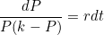
    \begin{equation*}\frac{dP}{P(k-P)}=r dt{\end{equation}

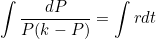
    \begin{equation*}\int \frac{dP}{P(k-P)}=\int r dt{\end{equation}

I am going to separate the denominator on the left hand side

\frac{1}{P(k-P)}=\frac{A}{P}+\frac{B}{k-P}
Hence,
\frac{1}{P(k-P)}=\frac{A(k-P)+BP}{P(k-P)}
1=A(k-P)+BP
When P=0,
1=Ak\Rightarrow A=\frac{1}{k}
When P=k,
1=BK\Rightarrow B=\frac{1}{k}

So our equation is,

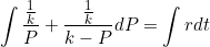
    \begin{equation*}\int \frac{\frac{1}{k}}{P}+\frac{\frac{1}{k}}{k-P} dP=\int r dt\end{equation}

    \begin{equation*}\frac{1}{k}\int \frac{1}{P}+\frac{1}{k-P} dP=\int r dt\end{equation}

    \begin{equation*}\int \frac{1}{P}+\frac{1}{k-P} dP=\int kr dt\end{equation}

    \begin{equation*}ln\lvert{P}\rvert-ln\lvert{k-P}\rvert=krt+c\end{equation}

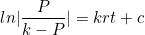
    \begin{equation*}ln\lvert{\frac{P}{k-P}\rvert=krt+c\end{equation}

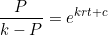
    \begin{equation*}\frac{P}{k-P}=e^{krt+c}\end{equation}

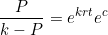
    \begin{equation*}\frac{P}{k-P}=e^{krt}e^{c} \end{equation}

When t=0, P=P_0,

    \begin{equation*}\frac{P_0}{k-P_0}=e^{c} \end{equation}

The equation is now

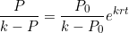
    \begin{equation*}\frac{P}{k-P}=\frac{P_0}{k-P_0}e^{krt}\end{equation}

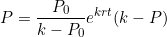
    \begin{equation*}P=\frac{P_0}{k-P_0}e^{krt}(k-P)\end{equation}

    \begin{equation*}P=k\frac{P_0}{k-P_0}e^{krt}-P\frac{P_0}{k-P_0}e^{krt}\end{equation}

    \begin{equation*}P+P\frac{P_0}{k-P_0}e^{krt}=k\frac{P_0}{k-P_0}e^{krt}\end{equation}

    \begin{equation*}P(1+\frac{P_0}{k-P_0}e^{krt})=k\frac{P_0}{k-P_0}e^{krt}\end{equation}

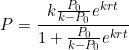
    \begin{equation*}P=\frac{k\frac{P_0}{k-P_0}e^{krt}}{1+\frac{P_0}{k-P_0}e^{krt}}\end{equation}

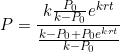
    \begin{equation*}P=\frac{k\frac{P_0}{k-P_0}e^{krt}}{\frac{k-P_0+P_0e^{krt}}{k-P_0}}\end{equation}

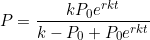
    \begin{equation*}P=\frac{kP_0e^{rkt}}{k-P_0+P_0e^{rkt}}\end{equation}

Divide by e^{rkt}

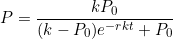
    \begin{equation*}P=\frac{kP_0}{(k-P_0)e^{-rkt}+P_0}\end{equation}

    \begin{equation*}}\frac{dP}{dt}=rP(k-P)\Longleftrightarrow P=\frac{kP_0}{(k-P_0)e^{-rkt}+P_0}\end{equation}

Proving the Maximum Rate of Increase Happens When P=\frac{k}{2}

    \begin{equation*}\frac{dP}{dt}=rP(k-P)\end{equation}

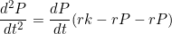
    \begin{equation*}\frac{d^2P}{dt^2}=r\frac{dP}{dt}(k-P)+rP(-\frac{dP}{dt})\end{equation}

    \begin{equation*}\frac{d^2P}{dt^2}=\frac{dP}{dt}(rk-rP-rP)\end{equation}

    \begin{equation*}\frac{d^2P}{dt^2}=0\end{equation}

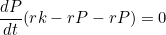
    \begin{equation*}\frac{dP}{dt}(rk-rP-rP)=0\end{equation}

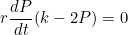
    \begin{equation*}r\frac{dP}{dt}(k-2P)=0\end{equation}

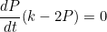
    \begin{equation*}\frac{dP}{dt}(k-2P)=0\end{equation}

    \begin{equation*}rP(k-P)(k-2P)=0\end{equation}

Hence P=k or P=\frac{k}{2}

(1)   \begin{equation*}\frac{d^3P}{dt^3}=\frac{dP^2}{dt^2}(rk-2rP)+\frac{dP}{dt}(-2\frac{dP}{dt})\end{equation*}

Substitute P=k into equation 1

    \begin{equation*}\frac{d^3P}{dt^3}=rk(k-k)(rk-2rk)(rk-2rk)-2(rk(k-k))^2=0\end{equation}

Hence, not a maximum.

Substitute P=\frac{k}{2} into equation 1

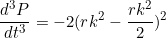
    \begin{equation*}\frac{d^3P}{dt^3}=rk(k-\frac{k}{2})(rk-2r\frac{k}{2})(rk-2r\frac{k}{2})-2(rk(k-\frac{k}{2}))^2=0\end{equation}

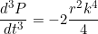
    \begin{equation*}\frac{d^3P}{dt^3}=-2(rk^2-\frac{rk^2}{2})^2\end{equation}

    \begin{equation*}\frac{d^3P}{dt^3}=-2\frac{r^2k^4}{4}\end{equation}

-2\frac{r^2k^4}{4}\le 0 For all values of P, r and k.

Hence maximum when P=\frac{k}{2}

We will look at a worked example in the next post.

Leave a Comment

Filed under Differential Equations, Differentiation, Implicit, Logistic Growth, Optimisation, Product Rule, Uncategorized, Year 12 Specialist Mathematics

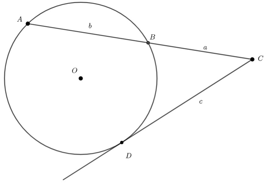
Intersecting Secant Theorem

CD is a tangent to the circle.

Prove c^2=a(a+b)

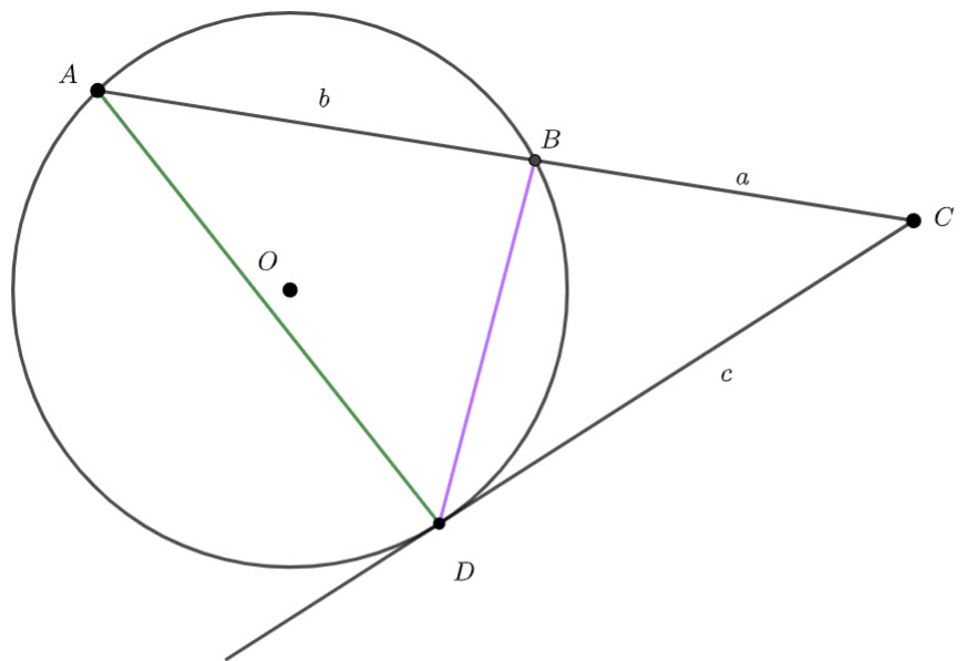
I am going to add two chords to the circle

Chord AD and BD are added

\angle{BDC}=\angle{CAD} (angles in alternate segments are congruent)
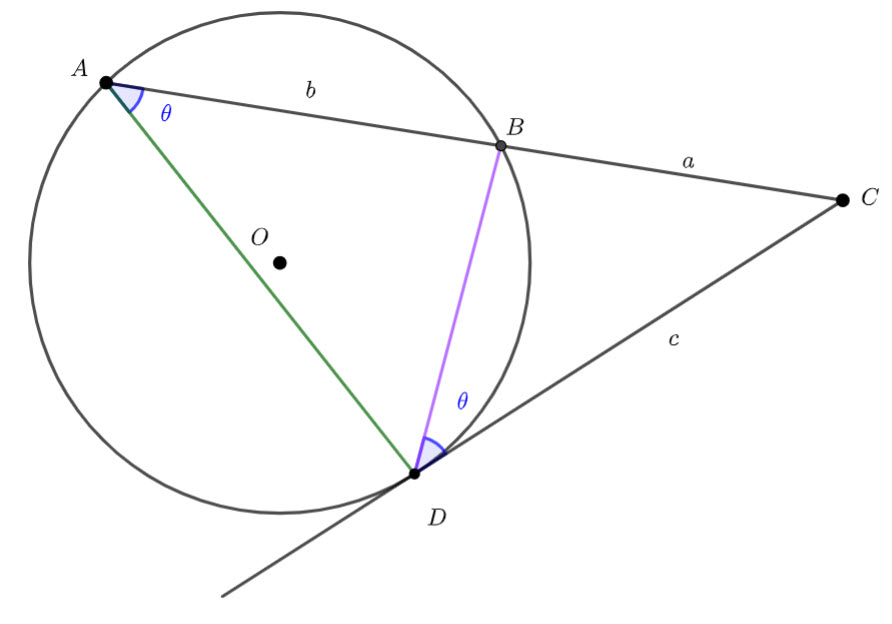
\angle{BCD}=\angle{DCA} (shared angle)

\therefore \Delta BDC\cong \Delta{DAC} (AA)

Hence

\frac{DC}{AC}=\frac{BC}{DC} (Corresponding sides in similar triangles)

\frac{c}{a+b}=\frac{a}{c}

\therefore c^2=a(a+b)

1 Comment

Filed under Circle Theorems, Geometry, Year 11 Specialist Mathematics