My Year 11 Specialist students have had an investigation which involves finding eigenvalues, eigenvectors and lines that are invariant under a particular linear transformation. This is not part of the course, but I feel for teachers who have to create new investigations every year.
Let’s find the eigenvalues and eigenvectors for matrix
We want to find such that
(1)
We solve
Hence and
When ,
Hence,
and the eigenvector is
When ,
Hence,
and the eigenvector is
Which means the invariant lines are and
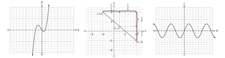
A quadrilateral with vertices on our lines
The vertices after they have been transformed – A and C remain in the same place (they are on the line)
The quadrilateral (purple) after the transformation
I was working on a question and involved 11 and I wondered what the divisibility rule was?
So then I had a bit of a think about it.
Let be a number divisible by . The
Now which is congruent to because , which is a multiple of 11.
Thus
Odd powers will be negative and even positive.
So if we start at one end of the number and add every second digit (i.e. first digit plus third digit plus fifth digit etc.) and then subtract the other digits (i.e. second digit, fourth digit, six digit, etc.), if that equals zero then the number is divisible by 11.
Arithmetic progressions (or arithmetic sequences) are sequences with a common difference (i.e. the same number is added or subtracted to get the next number in the sequence).
For example,
or
The term of an arithmetic progression is where is the first term and is the common difference.
i.e. For the sequence above,
An arithmetic series is the sum of the arithmetic progression.
For example, if the sequence is
then
The series is also a sequence and we are going to find the general term, .
which we can write as
Now, I am going to write that in reverse order (to make the next bit more obvious)
I am going to add the two versions of together
Each term has an and there are terms, so we now have . The terms, we going to group together
Which simplifies to and we have terms. So this part of the sum is
The unit square is rotated about the origin by anti-clockwise. (a) Find the matrix of this transformation. (b) Draw the unit square and its image on the same set of axes. (c) Find the area of the over lapping region.
Remember the general rotation matrix is
Hence
The unit square has co-ordinates
Unit Square
Transform the unit square
Unit Square and Transformed Unit Square
The overlapping area is the area of – the area of
We know because the diagonal of a square bisects the angle.
We know is a right angle as it’s on a straight line with the vertex of a square.
Two rectangular garden beds have a combined area of . The larger bed has twice the perimeter of the smaller and the larger side of the smaller bed is equal to the smaller side of the larger bed. If the two beds are not similar, and if all edges are a whole number of metres, what is the length, in metres, of the longer side of the larger bed? AMC 2007 S.14
Let’s draw a diagram
From the information in the question, we know
(1)
and
(2)
Equation becomes
As the sides are whole numbers, consider the factors of 40.
Remember
Perimeter Large
Perimeter Small
Comment
must be greater than
This one works
This one also works
not a whole number
Not possible
Not possible
Not possible
There are two possibilities
The large garden bed could be by and the smaller by (Area Perimeters and )
or
The large garden bed could be by and the smaller by (Area Perimeters and )


 (‘ones’)
 (‘tens’)
 (‘hundreds)
 (‘thousands’)
 the sum of powers of


 to base
  the first number is 1
 the second number is 1
 the third number is 0
 the fourth number is 0
 the fifth number is 0
 the sixth number is 1 and we have finished
 ?
?
 first number is zero
 second number is 1
 third number is 1
 fourth number is 1
 fifth number is 0
 sixth number is 0


 .
.


 such that


 and
and 
 ,
, 

 and the eigenvector is
 ,
, 

 and the eigenvector is
 and
and 


 be a number divisible by
  . The
. The 


 which is
  , which is a multiple of 11.
 divisible by


 term of an arithmetic progression is
  where
where  is the first term and
  is the common difference.


 .
.


 . The
. The 
 and we have


 anti-clockwise.


 – the area of
 because the diagonal of a square bisects the angle.
 is a right angle as it’s on a straight line with the vertex of a square.
 and
and  , hence


 . Then the distance the hour hand moves is
  (The angle between the hands at 2pm is
  )
) per minute, and the rate the minute hand moves is
  per minute.


 , the change in time is
  minutes and
  seconds. Hence the time is
  pm
pm
 . The larger bed has twice the perimeter of the smaller and the larger side of the smaller bed is equal to the smaller side of the larger bed. If the two beds are not similar, and if all edges are a whole number of metres, what is the length, in metres, of the longer side of the larger bed?


 and
and  )
)


 and
and  are equidistant from the origin. I.e.


 be the rotation matrix, then

 after it is rotated


 .
. is the midpoint of
  .
.
 is a point on the line.


 in terms of


 and
and 
 , which we can generalise to
 to
to 


 .
.


 are
are  and
and  .
.  is a reflection of
 is
is 


