This question is from Challenging Problems in Algebra
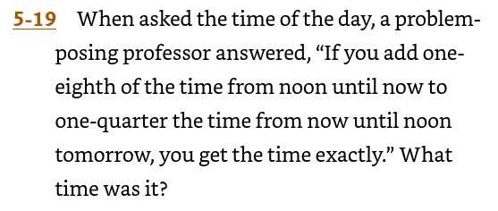
It’s the type of question students hate – “Who talks like that?”
Let  be the number of hours from noon.


Hence the time is 5:20pm
This question is from Challenging Problems in Algebra
It’s the type of question students hate – “Who talks like that?”
Let be the number of hours from noon.
Hence the time is 5:20pm
Filed under Algebra, Puzzles, Simplifying fractions, Solving Equations
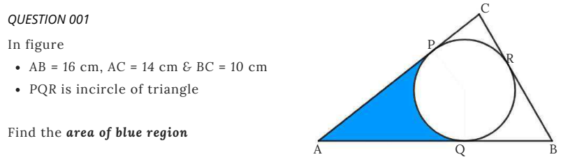
The blue shaded area is the area of triangles  and
and  subtract the sector
  .
.
We can use Heron’s law to find the area of the triangle 

where 

We also know the area of triangle  where
where  is the radius of the inscribed circle.
Hence,  and
and 
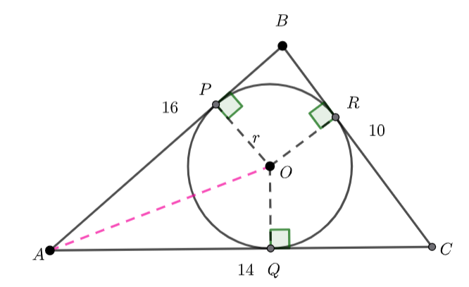
We know  , and
, and  – tangents to a circle are congruent.
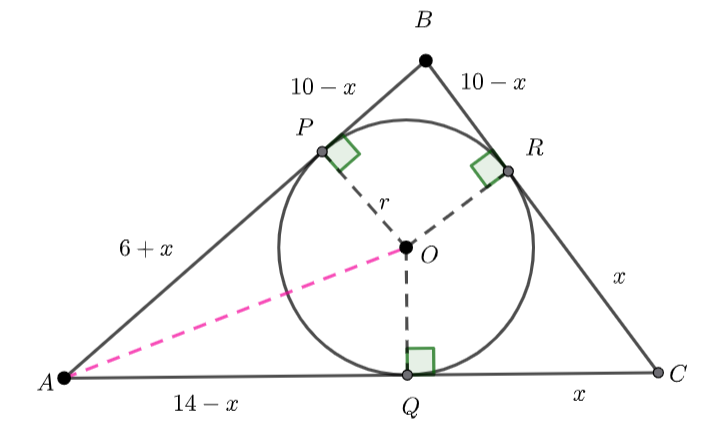

(1) 
(2) 
Area 
Area  Area
Area 
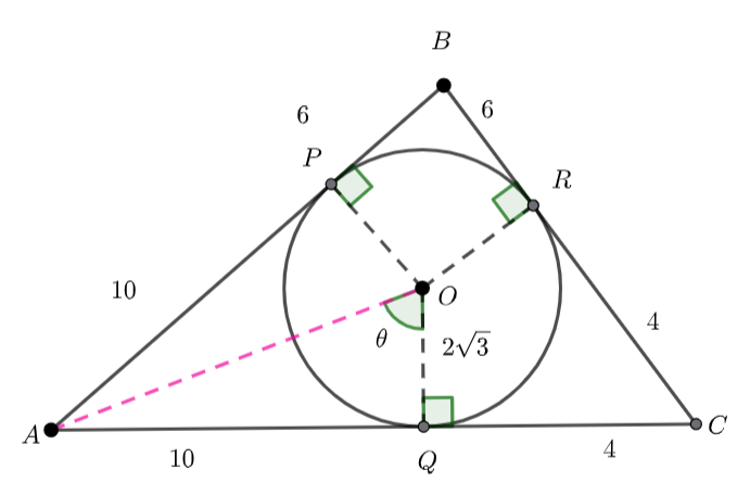


Area of sector 
Blue area = 


Where  is the semi-perimeter, and is the radius of the incircle.
 and
and  are tangents to the circle. And the radii are perpendicular to the tangents.
Add line segments  and
and  .
.
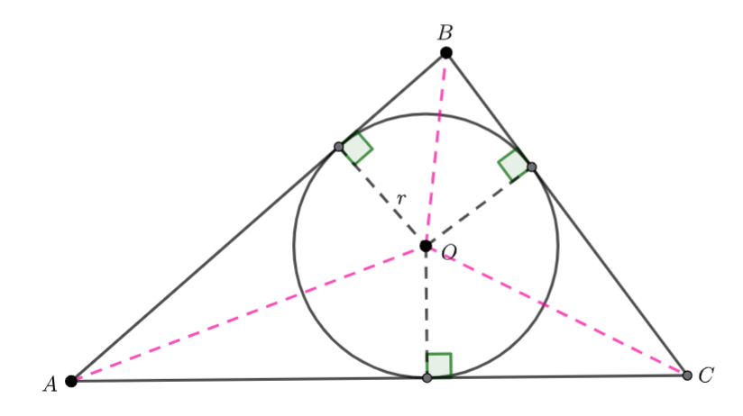
is split into three triangles,  and
and  .
.
Hence Area 


Remember 
Filed under Area, Finding an area, Geometry, Interesting Mathematics, Radius and Semi-Perimeter
Solve  for
for 
Remember the identity
(1) 
Hence

Now I have


 or
or 

 for
for 


Hence 
I usually choose to use synthetic division when factorising polynomials, but I know some teachers are unhappy when their students do this. So for completeness, here is my PDF for Polynomial Long Division.
In the diagram below,  and
and  lie on the circle with centre
  . If
. If  and
and  , determine with reasoning
  and
and 

We know  – radii of the circle.
Which means,  is isosceles and
  – equal angles isosceles triangle.
 – angle at the centre twice the angle at the circumference.


This means  – angles on a straight line are supplementary
 – equal angles isosceles triangle and the angle sum of a triangle.
 – angle at the circumference subtended by the same arc are congruent.

 – angles at the circumference subtended by the same arc are congruent.
 – equal angle isosceles triangle
Hence 
Completing the square is useful to
When completing the square we take advantage of perfect squares. For example, 
 and
and 
Put  into completed square form.
What perfect square has an  term?
term?

We don’t want  , we want
  , so subtract


What about a non-monic quadratic? For example,

Factorise the 

And continue as before
![2[(x+3)^2-9+\frac{11}{2}]=2[(x+3)^2-\frac{18}{2}+\frac{11}{2}]=2[(x+3)^2-\frac{7}{2}]=2(x+3)^2-7](https://www.racquelsanderson.com/wp-content/ql-cache/quicklatex.com-75a4ad924f4dac2900b0825b3dbc5eb1_l3.png "Rendered by QuickLaTeX.com")


![2[(x+\frac{7}{4})^2-(\frac{7}{4})^2-\frac{5}{2}]](https://www.racquelsanderson.com/wp-content/ql-cache/quicklatex.com-86decb178d67f6e763e3418b68dd4609_l3.png "Rendered by QuickLaTeX.com")
![2[(x+\frac{7}{4})^2-\frac{49}{16}-\frac{40}{16}]](https://www.racquelsanderson.com/wp-content/ql-cache/quicklatex.com-46cc98a61881eb23836f41e52a308e56_l3.png "Rendered by QuickLaTeX.com")
![2[(x+\frac{7}{4})^2-\frac{89}{16}]](https://www.racquelsanderson.com/wp-content/ql-cache/quicklatex.com-9c430d81a00ab51437da9037c1141aac_l3.png "Rendered by QuickLaTeX.com")


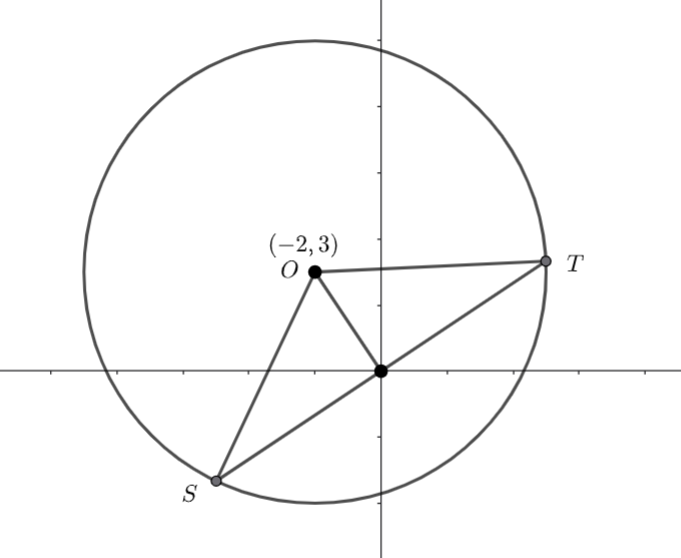
A circle has equation
(a) Find the centre and radius of the circle.
Pointsand
lie on the circle such that the origin is the midpoint of
.
(b) Show that
(a)We need to put the circle equation into completed square form


The centre is  and the radius is
  .
.
(b)Draw a diagram
We know  and
and  are radii of the circle. Hence
  is isosceles and the line segment from to the origin is perpendicular to .
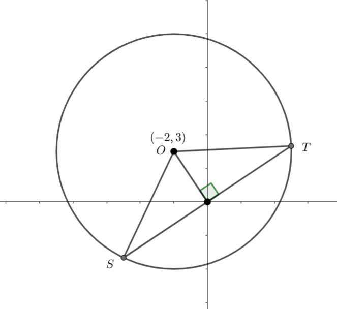
 and the distance from to the origin is

We can use Pythagoras to find the distance from the origin to .

Hence 
The Year 12 Mathematics Methods course doesn’t cover Integration by Parts, so they end up with questions like the following.
Determine the following:
(a)
(b)
Hence, determine the following integral by considering both parts (a) and (b)
(a) Use the product rule
(1) 
(b)
(2) 
I need to use equations  and to find
  .
.
The  terms need to vanish and I need
  of the
  terms.

(3) 
(4) 
Equation  plus equation
(5) 
Integrate both sides of the equation

By the fundamental theorem of calculus, we know
![(3e^{2x}sin(3x) \right)+2 \left (e^{2x}cos(3x) \right ]_0^{\frac{\pi}{2}}=\int_0^{\frac{\pi}{2}}13e^{2x}cos(3x) \enspace dx](https://www.racquelsanderson.com/wp-content/ql-cache/quicklatex.com-340dcf46fcda38d619ef2ee2af598ebd_l3.png "Rendered by QuickLaTeX.com")


Remember 

Let  , then
and  , then


Let  , then
and . then
![\int_0^{\frac{\pi}{2}}e^{2x}cos(3x) \enspace dx=-\frac{1}{2}+\frac{3}{2}(\frac{e^{2x}}{2}sin(3x)]_0^{\frac{\pi}{2}}-\int_0^{\frac{\pi}{2}} \frac{e^{2x}}{2}(3cos(3x)) \enspace dx)](https://www.racquelsanderson.com/wp-content/ql-cache/quicklatex.com-a21e419ffd82513840001a09eec6e482_l3.png "Rendered by QuickLaTeX.com")


Collect like terms (the integrals are like)


(1) 
My Year 12 Mathematics Methods students are getting ready for their exam, and questions using the above idea have created a bit of consternation. I am going to work through an example, and show why the ‘formula’ works.
Find
.
![\begin{equation*}=\frac{d}{dx} \left (\frac{4t^3}{3}+\frac{3t^2}{2} \right ]_2^{x^2}\end{equation}](https://www.racquelsanderson.com/wp-content/ql-cache/quicklatex.com-3591b5fb022549bc0a52bd97e02e58e3_l3.png "Rendered by QuickLaTeX.com")


(2) 
If we used ‘formula’

(3) 
We can see equation and are the same.

Remember 


